Model Selection Tests For Nested And Non-nested Regression Models

How to compare regression models that have all or some variables in common

Often, the regression modeler is faced with a choice among two or more competing models for the same problem. Goodness-of-fit measures such as R-squared (or pseudo-R-squared) and the F-test for regression analysis can be used to indicate how well an individual model fits the training data set, while AIC or BIC scores of the two models can be compared to see which one fits the data set better.

However, such tests by themselves cannot be used to decide if between two models A and B, one of them is clearly superior than the other in a statistically significant manner.

For instance, if model A has an adjusted R-squared value of 0.67 and model B reports an adjusted R-squared of 0.76, is the difference of 0.09 big enough to be statistically significant? Or was model A just unlucky to be trained on an ill-fitting data sample?

It is this problem that model selection tests are designed to address. Specifically, given two regression models A and B, a model selection test will help you arrive at a decision about whether A is better or B is better. As we’ll see, selecting a suitable model from a pair of candidate models can be an interesting exercise that sometimes ends in the acceptance or rejection of both models!

Overview of the model selection procedure

The process of model selection is based on the formation of two hypotheses H1 and H2 such that H1 favors model A and and H2 favors model B. The selection test consists of a formulation of a test statistic X (a random variable) which obeys a certain known probability distribution if one of the two hypotheses, say H1, is true. This distribution gives us the probability that H1 is true for different observed values of X. Once the value of this test statistic X is calculated, we can use X’s probability distribution to ‘read off’ the probability of H1 being true. We then accept or reject H1 based on whether this probability is respectively greater or lesser than some critical probability α.

Nested versus non-nested regression models

The nature of the model selection test depends on whether the two models A and B are nested versus non-nested.

If model B contains all the regression variables (and thus parameters) of model A plus at least one more, then A is considered to be nested within B. Model A is called the restricted (or constrained) model while B is called the unrestricted (or unconstrained) model. The following figure illustrates this situation:

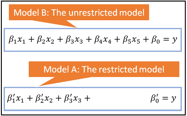
If the models are nested in the manner described above, tests such as the F-test for regression analysis and the Likelihood Ratio test can be used to select between the constrained and the unconstrained models.

The nice thing about the F test and the LR test is that as against adjusted R-squared, they can also be used for comparing nested nonlinear models. One more thing to note about them is that (and this holds true for adjusted R-squared and AIC also), it is necessary for the candidate models to have the same response variable y. One cannot use any of these tests to compare two models where model A has y as the response variable while model B has logy or sqrt(y) as the response variable.

When models A and B share only some of the regression variables or they do not share any regression variables, i.e. when they are not nested, the F-test and the LR test cannot be used for model selection. We need to look at a different set of model selection tests for comparing such non-nested models.

There is a vast amount of research literature available on model selection tests for non-nested models. We’ll examine one such test called the J test devised by Davidson and MacKinnon (1984) and we’ll illustrate its use in selecting between two non-nested regression models for a real world data set.

Illustration of the model selection procedure

The procedure for selecting a suitable model for a problem is best described using an example. In this chapter, we’ll compare the performance of two Fixed Effects Regression Models on a real world data set. The real-world data set we will use is a panel data set containing the Year-over-Year % growth in per capita GDP of seven countries measured from 1992 through 2014. Along with GDP growth data, the panel also contains Y-o-Y % growth data for Gross Capital Formation and per capita CO2 emissions for each country. The data set can be downloaded from this download link.

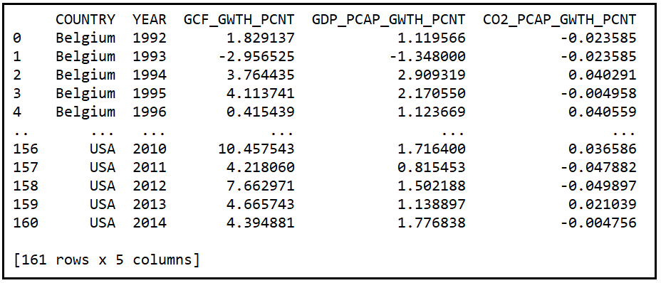
If you are new to the Fixed Effects model, I’ll suggest reviewing the chapter on Fixed Effects models. For the data set under consideration, you may think of an FE model as a linear regression model containing dummy variables (i.e. 1/0-valued variables), one dummy for each of the 7 countries in the data set. The dummies are supposed to capture the country-specific “effects”.

We’ll look at two competing FE models for the above data set.

Model A is an FE model in which we hypothesize that the per capita GDP changes from year to year are highly influenced (“explained”) by the changes in Gross Capital Formation.

Model B is also an FE model. Model B supposes that the per capita GDP change is explained, not so much by changes in Gross Capital Formation, as by yearly changes in CO2 emissions.

Both A and B being Fixed Effects models agree on representing the effects of the 7 countries in the data panel using 6 dummy variables. We use one less variable to avoid perfect multi-collinearity.

The equations for models A and B can be stated as follows:

For model A:

For model B:

In both equations, the subscript i refers to the ith row of the data set. The country-specific variables are dummy variables which have a value of 1 or 0 depending on whether the ith row relates to that country. β=[β_0,β_1,…β_7] is the vector of regression coefficients in model A while γ=[γ_0,γ_1,…γ_7] is the vector of coefficients in model B. Both β and γ vectors contain the intercept of regression β_0 and γ_0. In both models, ϵ_i is the error term for the ith row. The error term is the difference between the observed value of GDP_PCAP_GWTH_PCNT and its modeled value.

Using Python and statsmodels, let’s train A and B on the same data set using the classic OLS technique.

Let’s start by importing all the packages we will need:

import pandas as pd
import statsmodels.formula.api as smf
from patsy import dmatrices
import scipy.stats as st

Let’s define the units of interest in our Fixed Effects models:

unit_names = ['Belgium', 'CzechRepublic', 'France', 'Ireland', 'Portugal', 'UK', 'USA']

unit_names.sort()

Mark the column in the data set that contains the unit name:

unit_col_name='COUNTRY'

For model A, define the y and X variables. X does not yet include the dummies. We’ll add them soon.

y_var_name = 'GDP_PCAP_GWTH_PCNT'
X_var_names = ['GCF_GWTH_PCNT']

Load the panel data set of World Bank published development indicators into a Pandas Dataframe:

df_panel = pd.read_csv('wb_data_panel_4ind_7units_1992_2014.csv', header=0)

Print out the first 30 rows:

print(df_panel.head(30))

We see the following output:

Create the dummy variables, one dummy per country:

df_dummies = pd.get_dummies(df_panel[unit_col_name])

Join the dummies data frame with the rest of the data set:

df_panel_with_dummies = df_panel.join(df_dummies)

Let’s look at how the augmented data set looks like:

print(df_panel_with_dummies.head())

Now let’s construct the regression equation for model A. Recollect that model A uses Gross Capital Formation as one of the regression variables. Note that we are leaving out one dummy variable from the regression equation so as to avoid perfect multi-collinearity between the 7 dummy variables. The regression model’s intercept will contain the value of the coefficient for the omitted dummy variable (in our case, for USA):

model_a_expr = y_var_name + ' ~ '

i = 0

for X_var_name in X_var_names:
    if i > 0:
        model_a_expr = model_a_expr + ' + ' + X_var_name
    else:
        model_a_expr = model_a_expr + X_var_name
    i = i + 1

for dummy_name in unit_names[:-1]:
    model_a_expr = model_a_expr + ' + ' + dummy_name

Print out the regression equation (in Patsy syntax):

print('Regression expression for model A=\n' + model_a_expr)

We see the following output (the intercept is included silently by statsmodels during model creation):

Regression expression for model A=
GDP_PCAP_GWTH_PCNT ~ GCF_GWTH_PCNT + Belgium + CzechRepublic + France + Ireland + Portugal + UK

Build and train the Fixed Effects model A:

fe_model_a = smf.ols(formula=model_a_expr, data=df_panel_with_dummies)

fe_model_a_results = fe_model_a.fit()

Print out the training summary:

print(fe_model_a_results.summary())

We see the following output:

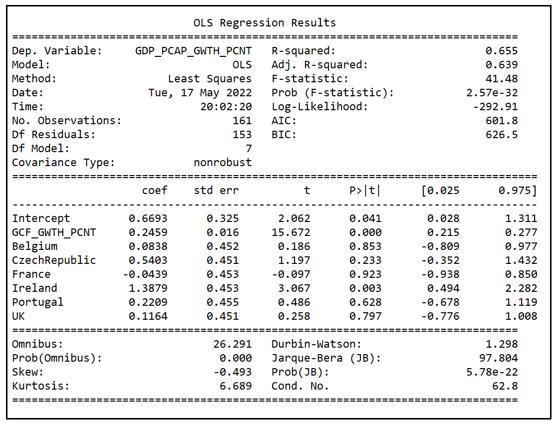
Let’s make a quick note of the adjusted R-squared reported by the model which is 0.639 and the p-value of the F-test which 2.57e-32. The p value is practically zero implying that the model did a much better job at explaining the variance in y than the mean model which is basically a flat line passing through the mean of y. This is good news.

Now, let’s repeat all of the above steps for Fixed Effects model B:

#Construct the regression equation.
X_var_names = ['CO2_PCAP_GWTH_PCNT']

model_b_expr = y_var_name + ' ~ '
i = 0
for X_var_name in X_var_names:
    if i > 0:
        model_b_expr = model_b_expr + ' + ' + X_var_name
    else:
        model_b_expr = model_b_expr + X_var_name
    i = i + 1

for dummy_name in unit_names[:-1]:
    model_b_expr = model_b_expr + ' + ' + dummy_name

print('Regression expression for model B=\n' + model_b_expr)

#Build and train model B
fe_model_b = smf.ols(formula=model_b_expr, data=df_panel_with_dummies)

fe_model_b_results = fe_model_b.fit()

#Print the model training summary
print(fe_model_b_results.summary())

We see the following output:

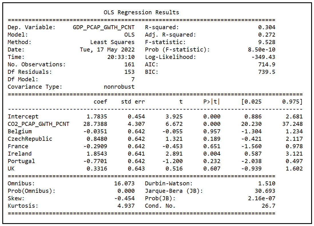
Note that the adjusted R-squared reported by model B is 0.272. Once again, the p value (8.5e-10) of the F-test is practically zero implying that model B has also performed a much better job of explaining the variance in y than the mean model.

A comparison of goodness-of-fit of models A and B

The adjusted R-squared (0.272) of model B is much smaller than that of model A (0.639). It appears to be a slam-dunk case for model A over model B. Other goodness-of-fit measures also seem to be favoring model A over model B. Log-likelihood of model A (-292.91) is higher than that of B (-349.43). AIC score of model A (601.8) is lower than that of model B (714.9). With AIC scores, a lower score is better.

In this case, it does not look like there is much competition between A and B. But imagine a scenario where model B’s R-squared, and Log-LL, and AIC score happened to be similar to those of A. In such a situation, how might one compare the fits of A and B?

Recollect that models A and B have only some of the regression variables in common, specifically, they have only the dummy variables in common. So A is not nested within B and neither is B within A. Thus, one cannot use the F-test or the Likelihood Ratio test to select between A and B.

In such a case, we may be able to use the J test. Let’s illustrate its usage.

The J test

The J test is based on the principle of composing what is known as a comprehensive model, which goes as follows:

1. We assume that models A and B are expected to be able to individually explain some of the variance in the response variable y.
2. Model A is described by the equation: y = Xβ + ϵ
3. Model B is described by the equation: y = Zγ + ϵ
4. We create a comprehensive model C that combines models A and B using a proportionately weighted-sum as follows:
   y = (1 — λ)Xβ + λZγ + ϵ, where λ varies from 0 to 1
5. Now here’s the key thing: If model A is able to explain all of the variance in y that model B was able to explain, plus some more, then model B is effectively encompassed within model A. We have no need for model B. In this situation, when you train the comprehensive model C on the data set, the fitted value of the coefficient λ should work out to zero.
6. On the other hand, if model B happens to be able to explain all of the variance in y that model A was individually able to explain, then model A is superfluous and the fitted coefficient λ ought to work out to 1.
7. In all other situations, fitted λ will be neither zero nor one, implying that each model A and B is able to individually explain some portion of the total variance in y that the other one isn’t able to explain. Neither model can be outright discarded in favor of the other one.
8. Interestingly, there is also a fourth scenario where after interchanging A and B in the comprehensive model C, λ still works out to zero. In this case, we end up rejecting both models A and B!

In the last two scenarios, the test is inconclusive in selecting between A and B.

The comprehensive model approach has a serious problem. Given the way λ is specified, it multiplies into the coefficients of models A and B. It is as such impossible to isolate λ from its interactions with the model’s coefficients thereby making λ practically unmeasurable.

The J test proposed by Davidson and MacKinnon addresses this problem while still preserving the spirit of the comprehensive model approach. What we do in the J test is to replace model B’s contribution to the comprehensive model with model B’s predicted (“fitted”) values of y. Doing so gives us the following updated equation for model C:

y = Xβ + Zγ_cap λ + ϵ, where λ varies from 0 to 1

We have replaced Zγ in the comprehensive model, with Zγ_cap where γ_cap is the vector of fitted coefficients of model B after B is fitted by itself on the data set.

The procedure for using the J test goes like this:

1. Fit model B on the data set by itself. This is the regression of y on Z, and from it we get the fitted coefficients γ_cap.
2. Run the training data set Z through the fitted model so as to produce the fitted model’s predictions y_cap=Zγ_cap.
3. Now, construct model C as an augmented version of model A in which one of the regression variables is y_cap. Thus, we are regressing y on X plus y_cap as follows:
   y = Xβ + y_capλ + ϵ
4. If in this augmented model, the coefficient λ of y_cap is found to be zero, then model B has not been able to explain any of the variance in y beyond what model A was able to explain. Therefore, model A subsumes model B and we select A in favor of B.
5. If λ in the augmented model is not zero, then model B has the capacity to explain some of the variance in y beyond what A was able to capture. In this case, we cannot select A over B. We’ll soon see what to do in such a situation.
6. We can also reverse the test by constructing model C as follows:
   y = Xβ_capλ + Zγ + ϵ
   i.e. we regress y on X, get the predictions y_cap=Xβ_cap from this model and add these predictions as a variable into the regression of y on Z. If the fitted coefficient of y_cap is zero, we conclude that A is unable to explain any variance in y beyond what B was able to explain. So we select B over A.

In the J test, it can come about the fitted λ is zero in both scenarios thereby indicating that neither A nor B are suitable for the data set.

Illustration of the J test

Let’s run the J test on the two Fixed Effects models we constructed earlier. In the language of the J test, we define X and Z as follows:

X is the regression variables matrix of the Fixed Effects model A:

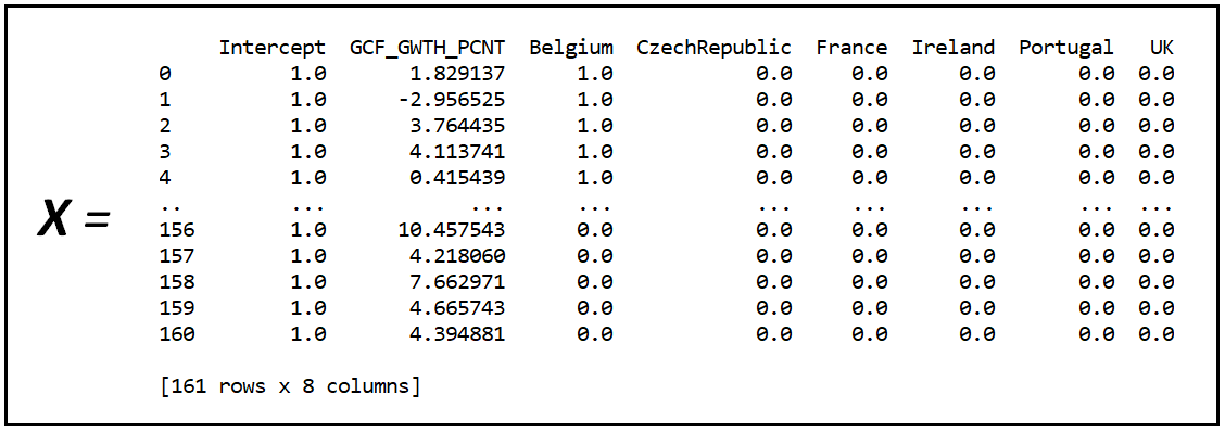
Z is the regression variable matrix of the Fixed Effects model B:

y is GDP_PCAP_GWTH_PCNT.

In the preceding section, we have already fitted model B on the data set. Let’s get its predictions on Z. To do so, we need to first carve out Z from the Pandas Data frame. Patsy’s dmatrices class will help us to do that using model B’s regression equation:

y_train, Z_train = dmatrices(model_b_expr, df_panel_with_dummies, return_type='dataframe')

Run the fitted model B on Z_train to get the predictions:

y_cap = fe_model_b_results.predict(Z_train)

Augment the data set by adding the predictions from model B:

df_panel_with_dummies['y_cap'] = y_cap

Now construct the comprehensive model (model C)’s regression equation. Recollect that model C’s expression is the following:

y = y_capλ +Xβ + ϵ

Where X is the regression matrix of model A, y_cap are the predictions from model B and ϵ is the error term of the regression.

X_var_names = ['y_cap', 'GCF_GWTH_PCNT']

comprehensive_model_expr = y_var_name + ' ~ '
i = 0
for X_var_name in X_var_names:
    if i > 0:
        comprehensive_model_expr = comprehensive_model_expr + ' + ' + X_var_name
    else:
        comprehensive_model_expr = comprehensive_model_expr + X_var_name
    i = i + 1

for dummy_name in unit_names[:-1]:
    comprehensive_model_expr = comprehensive_model_expr + ' + ' + dummy_name

print('Regression expression of the comprehensive model=\n' + comprehensive_model_expr)

We see the following output:

Regression expression of the comprehensive model=
GDP_PCAP_GWTH_PCNT ~ y_cap + GCF_GWTH_PCNT + Belgium + CzechRepublic + France + Ireland + Portugal + UK

Let’s build and train this model on the augmented data set:

comprehensive_model = smf.ols(formula=comprehensive_model_expr, data=df_panel_with_dummies)

comprehensive_model_results = comprehensive_model.fit()

print(comprehensive_model_results.summary())

We see the following results:

In the training summary, we see that except for the coefficients of y_cap and GCF_GWTH_PCNT, the coefficients of all variables are statistically insignificant (i.e. zero).

The coefficient of y_cap which is the proxy for model B in the comprehensive model is highly significant. This highlights an important finding: Model B carries some explanatory power within it that model A has not been able to capture. We should not entirely discard model B in favor of model A.

This decision runs contrary to what we had earlier set out to do by simply comparing the adjusted R-squared values and the Log-LL and AIC scores of both models.

But it begs the question, which variables in B carry this explanatory power beyond what model A has to offer? We can answer this question as follows:

The inclusion of y_cap — the proxy for B — in the comprehensive model has caused the coefficient of every single one of the variables that are common to A and B to become statistically insignificant in the fitted comprehensive model. Hence the only variables in B that could possibly have additional explanatory power are the ones not common with A, namely CO2_PCAP_GWTH_PCNT.

To test this hypothesis, we will add CO2_PCAP_GWTH_PCNT to model A so as to construct the following new model (we’ll call it model D):

Let’s fit model D on the training data set:

#Formulate model D by adding CO2_PCAP_GWTH_PCNT to model A
X_var_names = ['GCF_GWTH_PCNT', 'CO2_PCAP_GWTH_PCNT']

fe_model_d_expr = y_var_name + ' ~ '

i = 0

for X_var_name in X_var_names:
    if i > 0:
        fe_model_d_expr = fe_model_d_expr + ' + ' + X_var_name
    else:
        fe_model_d_expr = fe_model_d_expr + X_var_name
    i = i + 1

for dummy_name in unit_names[:-1]:
    fe_model_d_expr = fe_model_d_expr + ' + ' + dummy_name

print('Regression expression of model D=\n' + fe_model_d_expr)

#Build and train FE model D
fe_model_d = smf.ols(formula=fe_model_d_expr, data=df_panel_with_dummies)

fe_model_d_results = fe_model_d.fit()
print(fe_model_d_results.summary())

We see the following output:

Regression expression of model D=
GDP_PCAP_GWTH_PCNT ~ GCF_GWTH_PCNT + CO2_PCAP_GWTH_PCNT + Belgium + CzechRepublic + France + Ireland + Portugal + UK

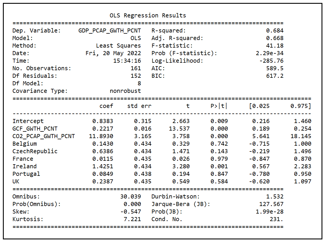
Let’s recall the training summary of model A:

Following is a comparison of the goodness-of-fit measures of Fixed Effects models A and D:

We see that all three goodness-of-fit measures are quite similar between models A and D, although D seems to have a slight edge over A.

We also note that model A is nested within D as model D contains all the variables of model A plus one more. Therefore, to know if model D is better than A in a statistically significant way we can use the F-test for regression analysis.

Using the F-test

We will use the F-test for testing the hypothesis that model D has produced a statistically better fit on the data set than model A.

Specifically, our two hypotheses for the F-test are as follows:

H1: Model D does not fit better than model A
H2: Model D fits better than model A

If H1 is found to be true, we will conclude that addition of CO2_PCAP_GWTH_PCNT to model A does not result in a better fit, and so we accept model A and reject D.

If H1 is falsified, we will conclude that addition of CO2_PCAP_GWTH_PCNT to model A leads to a statistically significant improvement in the goodness-of-fit. Hence, we will reject A in favor of D.

The test statistic for the F-test is as follows:

In the above formula,

RSS_a = residual sum of squares (also known as the residual errors) of fitted model A.
RSS_d = residual sum of squares of fitted model B.
k_a = number of parameters of model A (k_a=8)
k_d = number of parameters of model D (k_d=9)
N = number of rows in the training data set (N=161)

Let’s calculate the value of the F-statistic and compare its value with the critical F (1, 152) value at α=.05:

k_a = len(fe_model_a_results.params)
k_d = len(fe_model_d_results.params)
N = len(df_panel_with_dummies)
rss_a = fe_model_a_results.ssr
rss_d = fe_model_d_results.ssr

f_statistic = ((rss_a-rss_d)/(k_d-k_a))/(rss_d/(N-k_d))

print('F-statistic='+str(f_statistic))

alpha=0.05

f_critical_value=st.f.ppf((1.0-alpha), (k_d-k_a), (N-k_d))

print('F test critical value at alpha of 0.05='+str(f_critical_value))

We see the following output:

F-statistic=14.12366072014461
F test critical value at alpha of 0.05=3.9033664964061314

Since the calculated value of statistic (14.12) is much greater than the critical value (3.90), we reject H1 and accept H2 at a critical α of .05, i.e. at a (1 — .05)100%=95% confidence level.

Thus, we establish that Fixed Effects model D is indeed a better fitting model than Fixed Effects model A for the data set under consideration.

The Likelihood Ratio test

Since model A is nested within D, we could also use the LR test to compare the goodness-of-fits of the two models. Let’s use the LRT test and use its result to cross-verify the result of the F-test.

The test statistic of the Likelihood Ratio test is as follows:

In the above formula:

The restricted model is the one with fewer parameters. In our case, it is model A.

The unrestricted model is the one with the additional parameters, in our case, model D.

For both models, we calculate the maximized log-likelihood, subtract the one for the unrestricted model from the one for the restricted model and take negative 2 times the difference as the statistic.

The two competing hypotheses are the same as with the F-test namely:

H1: Model D does not fit better than model A
H2: Model D fits better than model A

Under the assumption that H1 is true, the LR test statistic is Chi-squared distributed with degrees of freedom equal to the difference between the number of parameters between the two models. In our case, this difference is (k_d — k_a)=(9–8)=1.

Let’s calculate the test statistic and compare its value with the critical Chi-squared(1) value at α of .05:

#Get the maximumed log likelihoods of models A and D
log_ll_a = fe_model_a_results.llf
log_ll_d = fe_model_d_results.llf

#Calculate the LR test statistic
lrt_statistic = -2*(log_ll_a - log_ll_d)
print('LRT-statistic='+str(lrt_statistic))

#Calculate the critical Chi-squared(1) value at alpha=0.05
alpha=0.05

chi2_critical_value=st.chi2.ppf((1.0-alpha), (k_d-k_a))

print('Chi-squared critical value at alpha of 0.05='+str(chi2_critical_value))

We see the following output:

LRT-statistic=14.305161418177136
Chi-squared critical value at alpha of 0.05=3.841458820694124

The test statistic’s value (14.31) is much greater than the critical Chi-squared(1) value of 3.84 at an α=.05 leading us to reject H1 and accept H2 that FE Model D produces a better goodness of fit than FE model A. The LR test agrees with the F-test.

Summary

We examined two competing non-nested Fixed Effects models A and B in their ability to explain the variance in per-capita GDP growth of 7 countries.

In FE model A, we hypothesized that per capital GDP growth is largely explained by the growth in per capita Gross Capital Formation (along with country-specific effects). In FE model B, we adopted a different hypothesis, presupposing that per capita GDP growth is explained by per capita growth in CO2 emissions (in addition to country-specific effects).

We trained both models on a panel data set to discover that model A appeared to produce a clearly superior fit.

However, when we used the J test to select between models A and B, we discovered that model B is also able to explain some of the variance in the dependent variable of regression beyond what model A is able to explain. Hence B cannot be entirely discarded in favor of A.

An analysis of the results of the J test revealed that it may benefit us to augment model A with the per capita CO2 emissions variable from model B.

We went ahead and did that thereby constructing a new model D and we proceeded to train D on the data set.

D’s goodness-of-fit, as evidenced by its adjusted R-squared, maximized Log-Likelihood and AIC scores was found to be quite similar to that of A, albeit with a slight edge over that of A. This raised the question: Could D have benefitted by chance from a benevolent data sample, i.e. a data panel that just happened to be tuned to D’s strengths?

Since A is nested within D, we were able to settle the matter by using the F-test for regression analysis and the Likelihood Ratio test to objectively compare the goodness of fit of A and D and to conclude that D is indeed a better fitting model than A.

Here’s the complete source code used in this chapter:

Citations and Copyrights

Data set

World Development Indicators data from World Bank under CC BY 4.0 license. Download link

Paper and Book Links

Pesaran, M. H. & Weeks, M., (1999). Non-nested Hypothesis Testing: An Overview, Cambridge Working Papers in Economics 9918, Faculty of Economics, University of Cambridge. Download link

Davidson, R., & MacKinnon, J. G. (1984). Model Specification Tests Based on Artificial Linear Regressions. International Economic Review, 25(2), 485–502. https://doi.org/10.2307/2526210

Images

All images are copyright Sachin Date under CC-BY-NC-SA, unless a different source and copyright are mentioned underneath the image.

PREVIOUS: The Chi-squared Test

NEXT: Testing The Assumptions Of the Cox Proportional Hazards Model Using Schoenfeld Residuals

UP: Table of Contents